12.4. Big O Orders
Big O notation commonly defines the following orders. These range from the lower orders, which describe code that, as the amount of data grows, slows down the least, to the higher orders, which describe code that slows down the most:
O(1), Constant Time (the lowest order)
O(log n), Logarithmic Time
O(n), Linear Time
O(n log n), N-Log-N Time
O(n2 ), Polynomial Time
O(2 n ), Exponential Time
O(n!), Factorial Time (the highest order)
Notice that big O uses the following notation: a capital O, followed by a pair of parentheses containing a description of the order. The capi- tal O represents order or on the order of. The n represents the size of the input data the code will work on. We pronounce O(n) as “big oh of n” or “big oh n.” You don’t need to understand the precise mathematic meanings of words like logarithmic or polynomial to use big O notation. I’ll describe each of these orders in detail in the next section, but here’s an oversimplified explanation of them:
O(1) and O(log n) algorithms are fast.
O(n) and O(n log n) algorithms aren’t bad.
O(n2 ), O(2 n ), and O(n!) algorithms are slow.
Certainly, you could find counterexamples, but these descriptions are good rules in general. There are more big O orders than the ones listed here, but these are the most common. Let’s look at the kinds of tasks that each of these orders describes. ## A Bookshelf Metaphor for Big O Orders In the following big O order examples, I’ll continue using the bookshelf metaphor. The n refers to the number of books on the bookshelf, and the big O ordering describes how the various tasks take longer as the number of books increases. ## O(1), Constant Time Finding out “Is the bookshelf empty?” is a constant time operation. It doesn’t matter how many books are on the shelf; one glance tells us whether or not the bookshelf is empty. The number of books can vary, but the runtime remains constant, because as soon as we see one book on the shelf, we can stop looking. The n value is irrelevant to the speed of the task, which is why there is no n in O(1). You might also see constant time written as O(c). ## O(log n), Logarithmic Logarithms are the inverse of exponentiation: the exponent 24 , or 2 × 2 × 2 × 2, equals 16, whereas the logarithm log 2 (16) (pronounced “log base 2 of 16”) equals 4. In programming, we often assume base 2 to be the logarithm base, which is why we write O(log n) instead of O(log2 2 n).
Searching for a book on an alphabetized bookshelf is a logarithmic time operation. To find one book, you can check the book in the middle of the shelf. If that is the book you’re searching for, you’re done. Otherwise, you can determine whether the book you’re searching for comes before or after this middle book. By doing so, you’ve effectively reduced the range of books you need to search in half. You can repeat this process again, checking the middle book in the half that you expect to find it. We call this the binary search algorithm, and there’s an example of it in “Big O Analysis Examples” later in this chapter.
The number of times you can split a set of n books in half is log 2 n. On a shelf of 16 books, it will take at most four steps to find the right one. Because each step reduces the number of books you need to search by one half, a bookshelf with double the number of books takes just one more step to search. If there were 4.2 billion books on the alphabetized bookshelf, it would still only take 32 steps to find a particular book.
Log n algorithms usually involve a divide and conquer step, which selects half of the n input to work on and then another half from that half, and so on. Log n operations scale nicely: the workload n can double in size, but the runtime increases by only one step. ## O(n), Linear Time Reading all the books on a bookshelf is a linear time operation. If the books are roughly the same length and you double the number of books on the shelf, it will take roughly double the amount of time to read all the books. The runtime increases in proportion to the number of books n. O(n log n), N-Log-N Time
Sorting a set of books into alphabetical order is an n-log-n time operation. This order is the runtime of O(n) and O(log n) multiplied together. You can think of a O(n log n) task as a O(log n) task that must be performed n times. Here’s a casual description of why.
Start with a stack of books to alphabetize and an empty bookshelf. Follow the steps for a binary search algorithm, as detailed in “O(log n), Logarithmic” on page 232, to find where a single book belongs on the shelf. This is an O(log n) operation. With n books to alphabetize, and each book taking log n steps to alphabetize, it takes n × log n, or n log n, steps to alphabetize the entire set of books. Given twice as many books, it takes a bit more than twice as long to alphabetize all of them, so n log n algo- rithms scale fairly well. In fact, all of the efficient general sorting algorithms are O(n log n): merge sort, quicksort, heapsort, and Timsort. (Timsort, invented by Tim Peters, is the algorithm that Python’s sort() method uses.) ## O(n 2 ), Polynomial Time Checking for duplicate books on an unsorted bookshelf is a polynomial time operation. If there are 100 books, you could start with the first book and compare it with the 99 other books to see whether they’re the same. Then you take the second book and check whether it’s the same as any of the 99 other books. Checking for a duplicate of a single book is 99 steps (we’ll round this up to 100, which is our n in this example). We have to do this 100 times, once for each book. So the number of steps to check for any duplicate books on the bookshelf is roughly n × n, or n 2 . (This approximation to n 2 still holds even if we were clever enough not to repeat comparisons.)
The runtime increases by the increase in books squared. Checking 100 books for duplicates is 100 × 100, or 10,000 steps. But checking twice that amount, 200 books, is 200 × 200, or 40,000 steps: four times as much work.
In my experience writing code in the real world, I’ve found the most com- mon use of big O analysis is to avoid accidentally writing an O(n 2 ) algorithm when an O(n log n) or O(n) algorithm exists. The O(n 2 ) order is when algo- rithms dramatically slow down, so recognizing your code as O(n 2 ) or higher should give you pause. Perhaps there’s a different algorithm that can solve the problem faster. In these cases, taking a data structure and algorithms (DSA) course, whether at a university or online, can be helpful.
We also call O(n 2 ) quadratic time. Algorithms could have O(n 3 ), or cubic time, which is slower than O(n 2 ); O(n 4 ), or quartic time, which is slower than O(n 3 ); or other polynomial time complexities. ## O(2 n ), Exponential Time Taking photos of the shelf with every possible combination of books on it is an exponential time operation. Think of it this way: each book on the shelf can either in be included in the photo or not included. Figure 13-1 shows every combination where n is 1, 2, or 3. If n is 1, there are two possible pho- tos: with the book and without. If n is 2, there are four possible photos: both books on the shelf, both books off, the first on and second off, and the sec- ond on and first off. When you add a third book, you’ve once again doubled the amount of work you have to do: you need to do every subset of two books that includes the third book (four photos) and every subset of two books that excludes the third book (another four photos, for 2 3 or eight photos). Each additional book doubles the workload. For n books, the number of photos you need to take (that is, the amount of work you need to do) is 2 n .
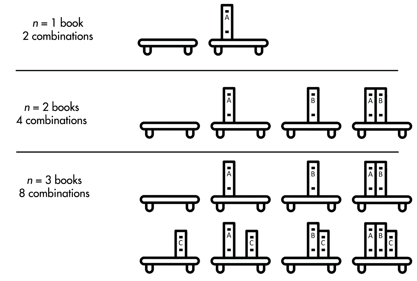
Figure 13-1: Every combination of books on a bookshelf for one, two, or three books
The runtime for exponential tasks increases very quickly. Six books require 2 6 or 32 photos, but 32 books would include 2 32 or more than 4.2 billion photos. O(2 n ), O(3 n ), O(4 n ), and so on are different orders ut all have exponential time complexity.
12.4.1. O(n!), Factorial Time
Taking a photo of the books on the shelf in every conceivable order is a factorial time operation. We call every possible order the permutation of n books. This results in n!, or n factorial, orderings. The factorial of a number is the multiplication product of all positive integers up to the number. For example, 3! is 3 × 2 × 1, or 6. Figure 13-2 shows every possible permutation of three books.

Figure 13-2: All 3! (that is, 6) permutations of three books on a bookshelf
To calculate this yourself, think about how you would come up with every permutation of n books. You have n possible choices for the first book; then n – 1 possible choices for the second book (that is, every book except the one you picked for the first book); then n – 2 possible choices for the third book; and so on. With 6 books, 6! results in 6 × 5 × 4 × 3 × 2 × 1, or 720 photos. Adding just one more book makes this 7!, or 5,040 photos needed. Even for small n values, factorial time algorithms quickly become impossible to complete in a reasonable amount of time. If you had 20 books and could arrange them and take a photo every second, it would still take longer than the universe has existed to get through every possible permutation.
One well-known O(n!) problem is the traveling salesperson conun- drum. A salesperson must visit n cities and wants to calculate the distance travelled for all n! possible orders in which they could visit them. From these calculations, they could determine the order that involves the short- est travel distance. In a region with many cities, this task proves impossible to complete in a timely way. Fortunately, optimized algorithms can find a short (but not guaranteed to be the shortest) route much faster than O(n!). ## Big O Measures the Worst-Case Scenario Big O specifically measures the worst-case scenario for any task. For exam- ple, finding a particular book on an unorganized bookshelf requires you to start from one end and scan the books until you find it. You might get lucky, and the book you’re looking for might be the first book you check. But you might be unlucky; it could be the last book you check or not on the bookshelf at all. So in a best-case scenario, it wouldn’t matter if there were billions of books you had to search through, because you’ll immediately find the one you’re looking for. But that optimism isn’t use- ful for algorithm analysis. Big O describes what happens in the unlucky case: if you have n books on the shelf, you’ll have to check all n books. In this example, the runtime increases at the same rate as the number of books.
Some programmers also use big Omega notation, which describes the best-case scenario for an algorithm. For example, a Ω(n) algorithm per- forms at linear efficiency at its best. In the worst case, it might perform slower. Some algorithms encounter especially lucky cases where no work has to be done, such as finding driving directions to a destination when you’re already at the destination.
Big Theta notation describes algorithms that have the same best- and worst-case order. For example, Θ(n) describes an algorithm that has linear efficiency at best and at worst, which is to say, it’s an O(n) and Ω(n) algo- rithm. These notations aren’t used in software engineering as often as big O, but you should still be aware of their existence.
It isn’t uncommon for people to talk about the “big O of the average case” when they mean big Theta, or “big O of the best case” when they mean big Omega. This is an oxymoron; big O specifically refers to an algo- rithm’s worst-case runtime. But even though their wording is technically incorrect, you can understand their meaning irregardless.
MORE TH A N E NOUGH M ATH TO DO BIG O
If your algebra is rusty, here’s more than enough math to do big O analysis:
Multiplication Repeated addition. 2 × 4 = 8, just like 2 + 2 + 2 + 2 = 8. With variables, n + n + n is 3 × n.
Multiplication notation Algebra notation often omits the × sign, so 2 × n is writ- ten as 2n. With numbers, 2 × 3 is written as 2(3) or simply 6.
The multiplicative identity property Multiplying a number by 1 results in that number: 5 × 1 = 5 and 42 × 1 = 42. More generally, n × 1 = n.
The distributive property of multiplication 2 × (3 + 4) = (2 × 3) + (2 × 4). Both sides of the equation equal 14. More generally, a(b + c) = ab + ac.
Exponentiation Repeated multiplication. 2 4 = 16 (pronounced “2 raised to the 4 th power is 16”), just like 2 × 2 × 2 × 2 = 16. Here, 2 is the base and 4 is the exponent. With variables, n × n × n × n is n 4 . In Python, we use the ** operator: 2 ** 4 evaluates to 16 .
The 1st power evaluates to the base 2 1 = 2 and 9999 1 = 9999. More gener- ally, n 1 = n.
The 0th power always evaluates to 1 2 0 = 1 and 9999 0 = 1. More generally,n 0 = 1.
Coefficients Multiplicative factors. In 3n 2 + 4n + 5, the coefficients are 3, 4, and 5. You can see that 5 is a coefficient because 5 can be rewritten as 5(1) and then rewritten as 5n 0.
Logarithms The inverse of exponentiation. Because 2 4 = 16, we know that log 2 (16) = 4. We pronounce this “the log base 2 of 16 is 4.” In Python, we use the math.log() function: math.log(16, 2) evaluates to 4.0 .
Calculating big O often involves simplifying equations by combining like terms. A term is some combination of numbers and variables multiplied together: in 3n 2 + 4n + 5, the terms are 3n 2 , 4n, and 5. Like terms have the same variables raised to the same exponent. In the expression 3n 2 + 4n + 6n + 5, the terms 4n and 6n are like terms. We could simplify and rewrite this as 3n 2 + 10n + 5.
Keep in mind that because n × 1 = n, an expression like 3n 2 + 5n + 4 can be thought of as 3n 2 + 5n + 4(1). The terms in this expression match with the big O orders O(n 2), O(n), and O(1). This will come up later when we’re drop- ping coefficients for our big O calculations.
These math rule reminders might come in handy when you’re first learn- ing how to figure out the big O of a piece of code. But by the time you finish “Analyzing Big O at a Glance” later in this chapter, you probably won’t need them anymore. Big O is a simple concept and can be useful even if you don’t strictly follow mathematical rules.