12.5. Determining the Big O Order of Your Code
To determine the big O order for a piece of code, we must do four tasks: identify what the n is, count the steps in the code, drop the lower orders, and drop the coefficients.
For example, let’s find the big O of the following readingList() function:
>>> def readingList(books):
>>>     print('Here are the books I will read:')
>>>     numberOfBooks = 0
>>>     for book in books:
>>>         print(book)
>>>         numberOfBooks += 1
>>>     print(numberOfBooks, 'books total.')
Recall that the n represents the size of the input data that the code works on. In functions, the n is almost always based on a parameter. The readingList() function’s only parameter is books , so the size of books seems like a good candidate for n, because the larger books is, the longer the func- tion takes to run.
Next, let’s count the steps in this code. What counts as a step is some- what vague, but a line of code is a good rule to follow. Loops will have as many steps as the number of iterations multiplied by the lines of code in the loop. To see what I mean, here are the counts for the code inside the readingList() function:
>>> def readingList(books):
>>>     print('Here are the books I will read:')   # 1 step
>>>     numberOfBooks = 0 # 1 step
>>>     for book in books: # n* step
>>>         print(book) # 1 step
>>>         numberOfBooks += 1 # 1 step
>>>     print(numberOfBooks, 'books total.') # 1 step
We’ll treat each line of code as one step except for the for loop. This line executes once for each item in books , and because the size of books is our n, we say that this executes n steps. Not only that, but it executes all the steps inside the loop n times. Because there are two steps inside the loop, the total is 2 × n steps. We could describe our steps like this:
>>> def readingList(books):
>>>     print('Here are the books I will read:')   # 1 step
>>>     numberOfBooks = 0 # 1 step
>>>     for book in books: # n*2 step
>>>         print(book) # (already counted)
>>>         numberOfBooks += 1 # (already counted)
>>>     print(numberOfBooks, 'books total.') # 1 step
Now when we compute the total number of steps, we get 1 + 1 + (n × 2) + 1. We can rewrite this expression more simply as 2n + 3.
Big O doesn’t intend to describe specifics; it’s a general indicator. Therefore, we drop the lower orders from our count. The orders in 2n + 3 are linear (2n) and constant (3). If we keep only the largest of these orders, we’re left with 2n.
Next, we drop the coefficients from the order. In 2n, the coefficient is 2. After dropping it, we’re left with n. This gives us the final big O of the readingList() function: O(n), or linear time complexity.
This order should make sense if you think about it. There are several steps in our function, but in general, if the books list increases tenfold in size, the runtime increases about tenfold as well. Increasing books from 10 books to 100 books moves the algorithm from 1 + 1 + (2 × 10) + 1, or 23 steps, to 1 + 1 + (2 × 100) + 1, or 203 steps. The number 203 is roughly 10 times 23, so the runtime increases proportionally with the increase to n. ## Why Lower Orders and Coefficients Don’t Matter We drop the lower orders from our step count because they become less significant as n grows in size. If we increased the books list in the previous readingList() function from 10 to 10,000,000,000 (10 billion), the number of steps would increase from 23 to 20,000,000,003. With a large enough n, those extra three steps matter very little.
When the amount of data increases, a large coefficient for a smaller order won’t make a difference compared to the higher orders. At a certain size n, the higher orders will always be slower than the lower orders. For example, let’s say we have quadraticExample() , which is O(n 2 ) and has 3n 2 steps. We also have linearExample() , which is O(n) and has 1,000n steps. It doesn’t matter that the 1,000 coefficient is larger than the 3 coefficient; as n increases, eventually an O(n 2 ) quadratic operation will become slower than an O(n) linear operation. The actual code doesn’t matter, but we can think of it as something like this:
>>> def quadraticExample(someData):# n is the size of someData
>>>     for i in someData:# n steps
>>>         for j in someData:# n steps
>>>             print('Something')# 1 step
>>>             print('Something')# 1 step
>>>             print('Something')# 1 step
>>>
>>>
>>> def linearExample(someData):# n is the size of someData
>>>     for i in someData:# n steps
>>>         for k in range(1000):# 1 * 1000 steps
>>>             print('Something') #(Already counted)
The linearExample() function has a large coefficient (1,000) compared to the coefficient (3) of quadraticExample() . If the size of the input n is 10, the O(n 2 ) function appears faster with only 300 steps compared to the O(n) function with 10,000 steps.
But big O notation is chiefly concerned with the algorithm’s per- formance as the workload scales up. When n reaches the size of 334 or greater, the quadraticExample() function will always be slower than the linearExample() function. Even if linearExample() were 1,000,000n steps, the quadraticExample() function would still become slower once n reached 333,334. At some point, an O(n 2 ) operation always becomes slower than an O(n) or lower operation. To see how, look at the big O graph shown in Figure 13-3. This graph features all the major big O notation orders. The x-axis is n, the size of the data, and the y-axis is the runtime needed to
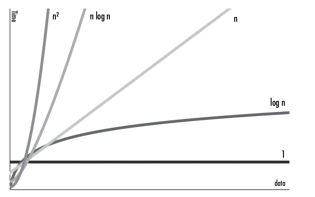
Figure 13-3: The graph of the big O orders
As you can see, the runtime of the higher orders grows at a faster rate than that of the lower orders. Although the lower orders could have large coefficients that make them temporarily larger than the higher orders, the higher orders eventually outpace them. ## Big O Analysis Examples Let’s determine the big O orders of some example functions. In these examples, we’ll use a parameter named books that is a list of strings of book titles.
The countBookPoints() function calculates a score based on the number of books in the books list. Most books are worth one point, and books by a certain author are worth two points:
>>> def countBookPoints(books):
>>>     points = 0# 1 step
>>>     for book in books: # n * steps in the loop
>>>         points += 1 # 1 step
>>>
>>>     for book in books: # n * steps in the loop
>>>         if 'by Al Sweigart' in book: # 1 step
>>>             points += 1 # 1 step
>>>     return points # 1 step
The number of steps comes to 1 + (n × 1) + (n × 2) + 1, which becomes 3n + 2 after combining the like terms. Once we drop the lower orders and coefficients, this becomes O(n), or linear complexity, no matter if we loop through books once, twice, or a billion times.
So far, all examples that used a single loop have had linear complexity, but notice that these loops iterated n times. As you’ll see in the next exam- ple, a loop in your code alone doesn’t imply linear complexity, although a loop that iterates over your data does.
This iLoveBooks() function prints “I LOVE BOOKS!!!” and “BOOKS ARE GREAT!!!” 10 times:
>>> def iLoveBooks(books):
>>>     for i in range(10):# 10 * steps in the loop
>>>         print('I LOVE BOOKS!!!')# 1 step
>>>         print('BOOKS ARE GREAT!!!')# 1 step
This function has a for loop, but it doesn’t loop over the books list, and it performs 20 steps no matter what the size of books is. We can rewrite this as 20(1). After dropping the 20 coefficient, we are left with O(1), or constant time complexity. This makes sense; the function takes the same amount of time to run, no matter what n, the size of the books list, is.
Next, we have a cheerForFavoriteBook() function that searches through the books list to look for a favorite book:
>>> def cheerForFavoriteBook(books, favorite):
>>>     for book in books:#n * steps in the loop
>>>         print(book)#1 step
>>>         if book == favorite:#1 step
>>>             for i in range(100):#100 * steps in the loop
>>>                 print('THIS IS A GREAT BOOK!!!')#1 step
The for book loop iterates over the books list, which requires n steps ultiplied by the steps inside the loop. This loop includes a nested for i m loop, which iterates 100 times. This means the for book loop runs 102 × n, or 102n steps. After dropping the coefficient, we find that cheerForFavoriteBook() is still just an O(n) linear operation. This 102 coefficient might seem rather large to just ignore, but consider this: if favorite never appears in the books list, this function would only run 1n steps. The impact of coefficients can vary so wildly that they aren’t very meaningful.
Next, the findDuplicateBooks() function searches through the bo
This function has a for loop, but it doesn’t loop over the books list, and it performs 20 steps no matter what the size of books is. We can rewrite this as 20(1). After dropping the 20 coefficient, we are left with O(1), or constant time complexity. This makes sense; the function takes the same amount of time to run, no matter what n, the size of the books list, is.
Next, we have a cheerForFavoriteBook() function that searches through the books list to look for a favorite book:
def cheerForFavoriteBook(books, favorite): for book in books: print(book) if book == favorite: for i in range(100): print(‘THIS IS A GREAT BOOK!!!’) # # # # # n * steps in the loop 1 step 1 step 100 * steps in the loop 1 step The for book loop iterates over the books list, which requires n steps ultiplied by the steps inside the loop. This loop includes a nested for i m loop, which iterates 100 times. This means the for book loop runs 102 × n, or 102n steps. After dropping the coefficient, we find that cheerForFavoriteBook() is still just an O(n) linear operation. This 102 coefficient might seem rather large to just ignore, but consider this: if favorite never appears in the books list, this function would only run 1n steps. The impact of coefficients can vary so wildly that they aren’t very meaningful. Next, the findDuplicateBooks() function searches through the books list (a linear operation) once for each book (another linear operation):
>>> def findDuplicateBooks(books):
>>>     for i in range(books): # n steps
>>>         for j in range(i + 1, books):# n steps
>>>             if books[i] == books[j]:# 1 step
>>>                 print('Duplicate:', books[i])# 1 step
The for i loop iterates over the entire books list, performing the steps inside the loop n times. The for j loop also iterates over a portion of the books list, although because we drop coefficients, this also counts as a linear time operation. This means the for i loop performs n × n operations—that is, n 2 . This makes findDuplicateBooks() an O(n 2 ) polynomial time operation.
Nested loops alone don’t imply a polynomial operation, but nested loops where both loops iterate n times do. These result in n 2 steps, implying an O(n 2 ) operation.
Let’s look at a challenging example. The binary search algorithm men- tioned earlier works by searching the middle of a sorted list (we’ll call it the haystack ) for an item (we’ll call it the needle ). If we don’t find the needle there, we’ll proceed to search the previous or latter half of the haystack , depend- ing on which half we expect to find the needle in. We’ll repeat this process, searching smaller and smaller halves until either we find the needle or we conclude it isn’t in the haystack . Note that binary search only works if the items in the haystack are in sorted order.
>>> def binarySearch(needle, haystack):
>>>     if not len(haystack):# 1 step
>>>         return None# 1 step
>>>     startIndex = 0# 1 step
>>>     endIndex = len(haystack) - 1# 1 step
>>>
>>>     haystack.sort()# ??? step
>>>
>>>     while start <= end: # 1 step
>>>         midIndex = (startIndex + endIndex) // 2# 1 step
>>>         if haystack[midIndex] == needle:# 1 step
>>> # Found the needle.
>>>             return midIndex# 1 step
>>>         elif needle < haystack[midIndex]:# 1 step
>>> # Search the previous half.
>>>             endIndex = midIndex - 1# 1 step
>>>         elif needle > haystack[mid]:# 1 step
>>> # Search the latter half.
>>>             startIndex = midIndex + 1# 1 step
Two of the lines in binarySearch() aren’t easy to count. The haystack .sort() method call’s big O order depends on the code inside Python’s sort() method. This code isn’t very easy to find, but you can look up its big O order on the internet to learn that it’s O(n log n). (All general sorting functions are, at best, O(n log n).) We’ll cover the big O order of several common Python functions and methods in “The Big O Order of Common Function Calls” later in this chapter.
The while loop isn’t as straightforward to analyze as the for loops we’ve seen. We must understand the binary search algorithm to determine how many iterations this loop has. Before the loop, the startIndex and endIndex cover the entire range of haystack , and midIndex is set to the midpoint of this range. On each iteration of the while loop, one of two things happens. If haystack[midIndex] == needle , we know we’ve found the needle , and the func- tion returns the index of the needle in haystack . If needle < haystack[midIndex] or needle > haystack[midIndex] , the range covered by startIndex and endIndex is halved, either by adjusting startIndex or adjusting endIndex . The number of times we can divide any list of size n in half is log 2 (n). (Unfortunately, this is simply a mathematical fact that you’d be expected to know.) Thus, the while loop has a big O order of O(log n).
But because the O(n log n) order of the haystack.sort() line is higher than O(log n), we drop the lower O(log n) order, and the big O order of the entire binarySearch() function becomes O(n log n). If we can guarantee that binarySearch() will only ever be called with a sorted list for haystack , we can remove the haystack.sort() line and make binarySearch() an O(log n) func- tion. This technically improves the function’s efficiency but doesn’t make the overall program more efficient, because it just moves the required sort- ing work to some other part of the program. Most binary search implemen- tations leave out the sorting step and therefore the binary search algorithm is said to have O(log n) logarithmic complexity. ## The Big O Order of Common Function Calls Your code’s big O analysis must consider the big O order of any functions it calls. If you wrote the function, you can just analyze your own code. But to find the big O order of Python’s built-in functions and methods, you’ll have to consult lists like the following.
This list contains the big O orders of some common Python operations for sequence types, such as strings, tuples, and lists:
s[i] reading and s[i] = value assignment O(1) operations.
s.append(value) An O(1) operation.
s.insert(i, value) An O(n) operation. Inserting values into a sequence(especially at the front)requires shifting all the items at indexes above i up by one place in the sequence.
s.remove(value) An O(n) operation. Removing values from a sequence (especially at the front) requires shifting all the items at indexes above I down by one place in the sequence.
s.reverse() An O(n) operation, because every item in the sequence must be rearranged.
s.sort() An O(n log n) operation, because Python’s sorting algorithm is O(n log n).
value in s An O(n) operation, because every item must be checked. for value in s: An O(n) operation.
len(s) An O(1) operation, because Python keeps track of how many items are in a sequence so it doesn’t need to recount them when passed to len() .
This list contains the big O orders of some common Python operations for mapping types, such as dictionaries, sets, and frozensets:
m[key] reading and m[key] = value assignment O(1) operations.
m.add(value) An O(1) operation.
value in m An O(1) operation for dictionaries, which is much faster than using in with sequences.
for key in m: An O(n) operation.
len(m) An O(1) operation, because Python keeps track of how many items are in a mapping, so it doesn’t need to recount them when passed to len() .
Although a list generally has to search through its items from start to finish, dictionaries use the key to calculate the address, and the time needed to look up the key’s value remains constant. This calculation is called a hash- ing algorithm, and the address is called a hash. Hashing is beyond the scope of this book, but it’s the reason so many of the mapping operations are O(1) constant time. Sets also use hashing, because sets are essentially dictionaries with keys only instead of key-value pairs.
But keep in mind that converting a list to a set is an O(n) operation, so you don’t achieve any benefit by converting a list to a set and then accessing the items in the set. ## Analyzing Big O at a Glance Once you’ve become familiar with performing big O analysis, you usually won’t need to run through each of the steps. After a while you’ll be able to just look for some telltale features in the code to quickly determine the big O order.
Keeping in mind that n is the size of the data the code operates on, here are some general rules you can use:
If the code doesn’t access any of the data, it’s O(1).
If the code loops over the data, it’s O(n).
If the code has two nested loops that each iterate over the data, it’s O(n 2 ).
Function calls don’t count as one step but rather the total steps of the code inside the function. See “Big O Order of Common Function Calls” on page 242.
If the code has a divide and conquer step that repeatedly halves the data,it’s O(log n).
If the code has a divide and conquer step that is done once per item in the data, it’s an O(n log n).
If the code goes through every possible combination of values in the n data, it’s O(2 n ), or some other exponential order.
If the code goes through every possible permutation (that is, ordering)of the values in the data, it’s O(n!).
If the code involves sorting the data, it will be at least O(n log n).
These rules are good starting points. But they’re no substitute for actual big O analysis. Keep in mind that big O order isn’t the final judgment on whether code is slow, fast, or efficient. Consider the following waitAnHour() function:
>>> import time
>>> def waitAnHour():
>>>     time.sleep(3600)
Technically, the waitAnHour() function is O(1) constant time. We think of constant time code as fast, yet its runtime is one hour! Does that make this code inefficient? No: it’s hard to see how you could have programmed a waitAnHour() function that runs faster than, well, one hour.
Big O isn’t a replacement for profiling your code. The point of big O notation is to give you insights as to how the code will perform under increasing amounts of input data. ## Big O Doesn’t Matter When n Is Small, and n Is Usually Small Armed with the knowledge of big O notation, you might be eager to ana- lyze every piece of code you write. Before you start using this tool to ham- mer every nail in sight, keep in mind that big O notation is most useful when there is a large amount of data to process. In real-world cases, the amount of data is usually small.
In those situations, coming up with elaborate, sophisticated algorithms with lower big O orders might not be worth the effort. Go programming language designer Rob Pike has five rules about programming, one of which is: “Fancy algorithms are slow when ‘n’ is small, and ‘n’ is usually small.” Most software developers won’t be dealing with massive data centers or complex calculations but rather more mundane programs. In these circumstances, running your code under a profiler will yield more concrete information about the code’s performance than big O analysis.